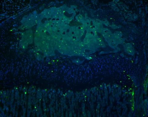
TUNEL assay (Dead End Fluorimetric Kit, Promega)

Sample preparation

sacrifice the animals and dissect knee samples
fix in 10% neutral buffered formalin(Sigma) over 48h in the fridge
decalcify in 20% EDTA pH7.4 for 2 weeks (shaking)
wax embed and section (6um sections)

Note

in order to generate statistically robust data, use 3 animals per genotype, 3 sections per animal (from different anatomically matched regions in the knee), 3 sections per slide.

original protocol files:

Staining steps

dewax in xylene 2 x 5min

. ↓

100% EtOH 5min

. ↓
100% EtOH 3min

. ↓

90% EtOH 3min

. ↓
70% EtOH 3min

. ↓
50% EtOH 3min

. ↓

0.85% NaCl 5min

. ↓

1x PBS (rocker) 5min (from here on, do not let the sections dry!)

. ↓

4% methanol-free formaldehyde (Fisher Scientific) in PBS 15min

. ↓

1x PBS (rocker) 2x5min

. ↓

citric buffer boil (in a glass jar; 10mM citric acid, 0.05% Tween 20, pH 6.0; microwave at 800W for 4min, 400W for 4min and 200W for 4min, allow to cool down on the bench)

. ↓

1x PBS (rocker) 5min

. ↓

4% methanol-free formaldehyde in PBS 5min

. ↓

1x PBS 5min

. ↓

draw around the section with ImmEdge pen.

keep the slides in a darkened humidified chamber during all incubations

. ↓

100ul equilibration buffer 5-10min

. ↓

50ul TdT per section, 37ºC 1h

. ↓

stop the reaction in 2xSSC 15min

. ↓

1x PBS 3x5min

. ↓

mount in Vectashield with DAPI (Vector Labs)

Modifications

proteinase K unmasking in the original protocol was replaced with citric buffer boil, as proteinase K is known to generate false positives[1][2][3]

end result: nuclei showing in DAPI filter, FITC positive TUNEL positive cells

Data analysis

count TUNEL positive cells (FITC) in the growth plate zones and present them as a percentage of all cells (FITC and DAPI) in each zone
use One Way ANOVA to statistically analyse the data

Notes on image aquisition

Images should be taken at the right magnification, allowing identification of individual cells in each zone of the growth plate. Analysis should be perormed per channel (blue separately from green).

Procedure

Watershed algorithm can be used both in ImageJ or Fiji. Make sure java is up to date on the computer as this is a java applet.

To quantify DAPI positive cells open the file and select the zone of interest:

Clear the outline leaving only the zone of interest:

For DAPI and other fluorescence images, invert the colours:

Convert the image into an 8-bit version:

Adjust brightness and contrast (clicking “Auto” and then “Apply” is often enough):

Activate the watershed plugin:

There are certain parameters which need to be set before the analysis:

Radius indicates the predicted radius of the particles to be measured. It works well at 0.5 for the resting and proliferative zones and 1.0 for the hypertrophic zone (larger cells). Min/max level indicates the intensity of greyness which is still recognised as a particle. 0 to 200 is a good setting for the general DAPI staining. If the staining is faint and not enough cells are picked out, in particular for the hypertrophic zone, increase max to 210-220. If too many cells/particles are counted, reduce the max down to 175.

Select “8-connected” particles for the analysis. This accounts for the fact that ellipsoid shapes which will be counted can be touching but will still be included in the analysis (a function which the regular particle counter plugin in ImageJ is lacking):